Optimization Rule in Deep Neural Networks

In machine learning, optimizers and loss functions are two fundamental components that help improve a model’s performance.

• A loss function evaluates a model’s effectiveness by computing the difference between expected and actual outputs. Common loss functions include log loss, hinge loss and mean square loss.
• An optimizer improves the model by adjusting its parameters (weights and biases) to minimize the loss function value. Examples include RMSProp, ADAM and SGD (Stochastic Gradient Descent).

The optimizer’s role is to find the best combination of weights and biases that leads to the most accurate predictions.

Gradient Descent

Gradient Descent is a popular optimization method for training machine learning models. It works by iteratively adjusting the model parameters in the direction that minimizes the loss function.

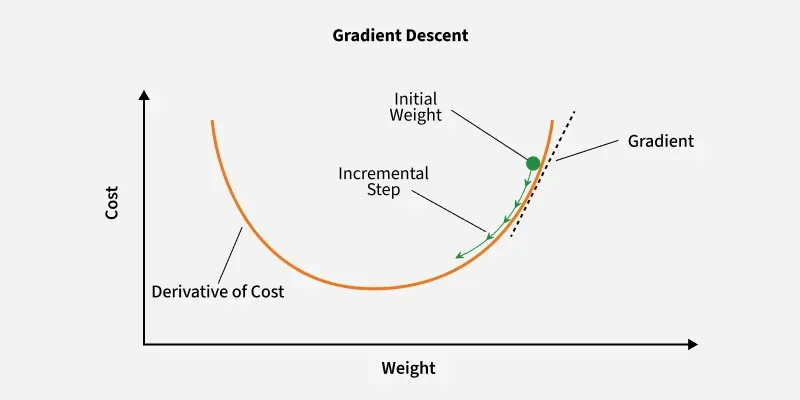
Gradient Descent

Key Steps in Gradient Descent

1. Initialize parameters: Randomly initialize the model parameters.
2. Compute the gradient: Calculate the gradient (derivative) of the loss function with respect to the parameters.
3. Update parameters: Adjust the parameters by moving in the opposite direction of the gradient, scaled by the learning rate.

Formula:

${\theta }_{(k+1)}={\theta }_k-\alpha \nabla J({\theta }_k)$

where:

• ${\theta }_{(k+1)}$ is the updated parameter vector at the $(k+1{)}^{th}$ iteration.
• ${\theta }_k$ is the current parameter vector at the kth iteration.
• $\alpha$ is the learning rate, which is a positive scalar that determines the step size for each iteration.
• $\nabla J({\theta }_k)$ is the gradient of the cost or loss function J with respect to the parameters ${\theta }_k$

Gradient Descent with Armijo Goldstein Condition

This variant ensures that the step size is large enough to effectively reduce the objective function, using a line search that satisfies the Armijo condition.

Condition:

$f(x^{t-1}+\alpha \nabla f(x^{t-1}))-f(x^{t-1})\ge c\alpha ||\nabla f(x^{t-1})|{|}^2$

Where:

• $\alpha$ is the step size.
• $c$ is a constant between 0 and 1.

Gradient Descent with Armijo Full Relaxation Condition

Incorporates both first and second derivatives (Hessian matrix) to determine a more optimal step size for the update.

Condition:

$f(x^{t-1}+\alpha \nabla f(x^{t-1}))-f(x^{t-1})\ge c\alpha ||\nabla f(x^{t-1})|{|}^2+\frac{b}{2}{\alpha }^2\nabla f(x^{t-1}{)}^{T}H(x)\nabla f(x^{t-1})$

Where:

• $H(x)$ is the Hessian matrix.
• $c$ and $b$ are constants between 0 and 1.

Variants of Gradient Descent

1. Stochastic Gradient Descent (SGD)

Stochastic Gradient Descent (SGD) updates the model parameters after each training example, making it more efficient for large datasets compared to traditional Gradient Descent, which uses the entire dataset for each update.

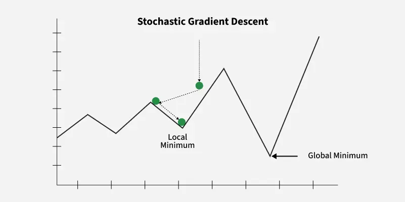
Stochastic Gradient Descent

Steps:

1. Select a training example.
2. Compute the gradient of the loss function.
3. Update the model parameters.

Advantages: Requires less memory and may find new minima.

Disadvantages: Noisier, requiring more iterations to converge.

2. Mini Batch Gradient Descent

Mini-batch gradient descent consists of a predetermined number of training examples, smaller than the full dataset. This approach combines the advantages of the previously mentioned variants.

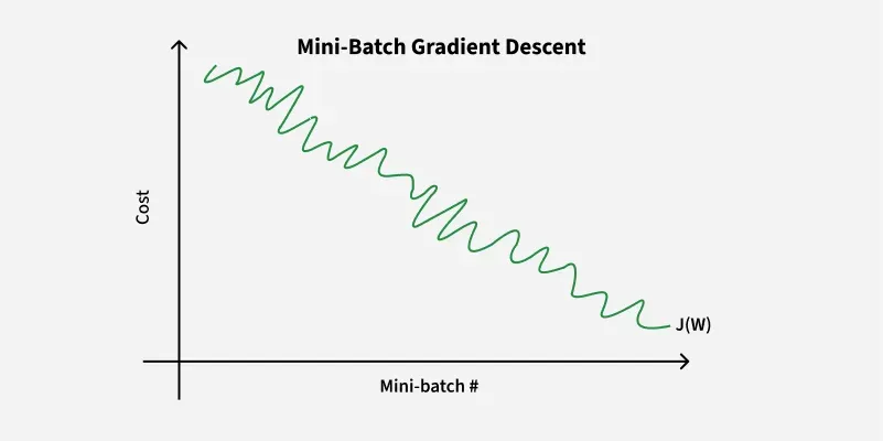
Mini-Batch Gradient Descent

In one epoch, following the creation of fixed-size mini-batches, we execute the following steps:

1. Select a mini-batch.
2. Compute the mean gradient of the mini-batch.
3. Apply the mean gradient obtained in step 2 to update the model’s weights.
4. Repeat steps 1 to 2 for all the mini-batches that have been created.

Advantages: Requires medium amount of memory and less time required to converge when compared to SGD

Disadvantage: May get stuck at local minima

3. SGD with Momentum

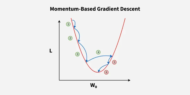
Momentum-Based Gradient Descent

Momentum helps accelerate convergence by smoothing out the noisy gradients of SGD, thus reducing fluctuations and improving the speed of convergence.

$v_{(t+1)}=\beta \ast v_t+(1-\beta )\ast \nabla J({\theta }_t)$

Where:

• $v_t$ is the momentum at time $t$.
• $\beta$ is the momentum coefficient.
• $\nabla J({\theta }_t)$ is the gradient at time $t$.

Then, the model parameters are updated using:

${\theta }_{(t+1)}={\theta }_t-\alpha \ast v_{(t+1)}$

Advantages: Mitigates oscillations, reduces variance and faster convergence.

Disadvantages: Requires tuning the momentum coefficient $\beta$.

Advanced Optimizers

1. AdaGrad

AdaGrad adapts the learning rate for each parameter based on the historical gradient information. The learning rate decreases over time, making AdaGrad effective for sparse features.

${\theta }_{(t+1)}={\theta }_t-\frac{\alpha }{\sqrt{G_t+\epsilon }}\ast \nabla J({\theta }_t)$

Where:

• $G_t$ is the sum of squared gradients.
• $\epsilon$ is a small constant to avoid division by zero.

Advantages: Adapts the learning rate, improving training efficiency.

Disadvantages: Learning rate decays too quickly, causing slow convergence.

2. RMSProp

RMSProp improves upon AdaGrad by introducing a decay factor to prevent the learning rate from decreasing too rapidly.

$E[g^2{]}_t=\gamma \ast E[g^2{]}_{(t-1)}+(1-\gamma )\ast (\nabla J({\theta }_t){)}^2$

${\theta }_{(t+1)}={\theta }_t-\frac{\alpha }{\sqrt{E[g^2{]}_t+\epsilon }}\ast \nabla J({\theta }_t)$

Where:

• $\gamma$ is the decay rate.
• $E[g^2{]}_t$ is the exponentially moving average of squared gradients.

Advantages: Prevents excessive decay of learning rates.

Disadvantages: Computationally expensive due to the additional parameter.

3. Adam (Adaptive Moment Estimation)

Adam combines the advantages of Momentum and RMSProp. It uses both the first moment (mean) and second moment (variance) of gradients to adapt the learning rate for each parameter.

1. Update the first moment: $m_t={\beta }_1\ast m_{(t-1)}+(1-{\beta }_1)\ast \nabla J({\theta }_t)$
2. Update the second moment: $v_t={\beta }_2\ast v_{(t-1)}+(1-{\beta }_2)\ast (\nabla J({\theta }_t){)}^2$
3. Bias correction: ${\hat{m}}_t=\frac{m_t}{1-{\beta }_1^t},{\hat{v}}_t=\frac{v_t}{1-{\beta }_2^t}$
4. Update parameters: ${\theta }_{(t+1)}={\theta }_t-\frac{\alpha }{\sqrt{{\hat{v}}_t+\epsilon }}\ast {\hat{m}}_t$

Where:

• ${\beta }_1$ and ${\beta }_2$ are the decay rates for the first and second moments.
• $\epsilon$ is a small constant to prevent division by zero.

Advantages: Fast convergence.

Disadvantages: Requires significant memory due to the need to store first and second moment estimates.

Comparison of Optimizers

Optimizer	Advantages	Disadvantages
SGD	Simple, easy to implement	Slow convergence, requires tuning
Mini-Batch SGD	Faster than SGD	Computationally expensive, stuck in local minima
SGD with Momentum	Faster convergence, reduces noise	Requires careful tuning of β
AdaGrad	Adaptive learning rates	Decays too fast, slow convergence
RMSProp	Prevents fast decay of learning rates	Computationally expensive
Adam	Fast, combines momentum and RMSProp	Memory-intensive, computationally expensive

Each optimizer has its own strengths and weaknesses. The choice of optimizer depends on the specific problem, dataset characteristics and the computational resources available. Adam is often the default choice due to its robust performance, but each situation may call for a different optimizer to achieve optimal results.